
Economist John Adams and Analyst Martin North discuss the recent RBA speech on Unconventional Monetary Policy: Some Lessons From Overseas.
Tag: RBA
Wages Lower For Longer
In the RBA’s Governor’s speech last night there was a reference to lower wages growth for longer, referring back to an earlier outing by Guy Debelle, Deputy Governor.
Debelle’s speech at Australian Council of Social Service (ACOSS) National Conference revealed at least to me that the RBA has no real idea as to why wages growth is so slow. They appear to have all but accepted it will be so. ” This increase in labour supply has meant that the strong employment outcomes in recent years has not generated the pick-up in wages growth that might otherwise have occurred. At the same time, I have highlighted the increased prevalence of wages growth in the 2s across the economy”.
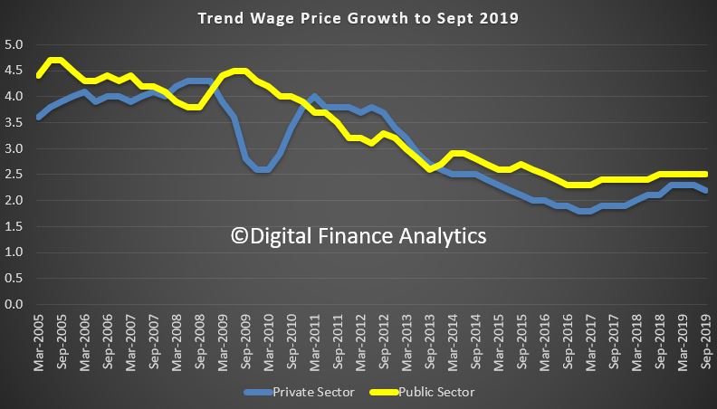
We think the structural changes to the labour market (gig jobs, part-time work, multiple-jobs, etc) plus technological changes and globalisation all have a role to play. And the migration factors and temporary working visas are also playing into the mix. Finally, the balance between employee and employer seems to have shifted. Public sector wages are a little stronger.
He said: Over much of the past three years, employment has grown at a healthy annual pace of 2½ per cent. This has been faster than we had expected, particularly so, given economic growth was slower than we had expected. Employment growth has also been faster than the working-age population has been growing. As a result, the share of the Australian population employed is around its all-time high, which is a good outcome. Normally, we would have expected this strong employment growth to lead to a decline in the unemployment rate. But the unemployment rate has turned out to be very close to what we had expected and has moved sideways around 5¼ per cent for some time now.
So what is going on here? Strong employment growth but little change in the unemployment rate means that the strength in labour demand has been met by strong growth in labour supply. This increase in labour supply has come from more people joining the labour force and from some of those with jobs putting off leaving the labour force. These trends have been particularly pronounced for females aged between 25 and 54 and older workers of both sexes.
The surprising strength in labour supply has been one of the factors that has contributed to wages growth being slower than we had expected. But at the same time, the lower growth in wages has probably contributed to the strength in employment growth. My undergraduate honours thesis at Adelaide Uni examined the aggregate labour demand curve in Australia which was a much debated topic at the time.[1] So more than 30 years on, I will discuss similar issues today.
I will look at the rise in participation rates of females and older workers and discuss some of the factors that have been contributing to it. I will also look briefly at what jobs have been created. In doing so, I will make use of the micro data in the monthly labour force survey (LFS) as well as micro data from the HILDA survey.[2] That is, we are examining the micro data to understand the macro trends in the labour market.
By and large, the new jobs created over the past few years have been representative of the existing stock of jobs. There have been low wage and high wage, lower skilled and higher skilled jobs created, but about average on both counts. The jobs growth has been in household services jobs such as health care, social assistance and, education, as well as in business services. Two-thirds of the employment growth over the past two years has been in full-time jobs.
Then I will look at wages growth and show that the lower average wage outcomes of the past few years have reflected the increased prevalence of wages growth in the 2s across the economy.
Finally, I will look forward and talk about the RBA’s forecasts for the labour market. Two of the critical influences on that forecast are how much further labour supply will increase and how entrenched are wage outcomes.
Participation
An increase in the number of people in employment can be met either by an increase in people entering from outside the labour market or a decline in unemployment. The increase in people coming from outside the labour force, causing an increase in the participation rate, is known as an ‘encouraged worker’ effect – when economic conditions improve, there is a tendency for people to enter or defer leaving the workforce.[3] Historically more of the increase in employment has translated into a reduction in the unemployment rate than by a rise in the participation rate.
However, the past couple of years have been unusual. The increase in employment has been met disproportionately by an increase in the number of people participating in the labour force (Graph 1). The share of the population participating in the labour force is at a record high. The two main groups contributing to this rise in participation are females and older workers. I will discuss each of these in turn and some of the forces driving the outcomes over both the recent past and from a longer perspective. An understanding of these forces can help us assess how much further these trends are likely to continue.
Female participation
Female employment growth has accounted for two-thirds of employment growth over the past year. The female participation rate is now at its highest rate, and the gap between female and male participation is now the narrowest it has ever been (Graph 2).
The female participation rate has steadily increased over recent decades (from 40 per cent in 1970 to 61 per cent in 2019), and a similar upward trend is evident across other advanced economies. Changing societal norms and rising educational attainment have contributed to more women moving into paid employment or employment outside the home. Female participation has also been influenced by the increasing flexibility of working-time arrangements, the availability and cost of child care and policies such as parental leave.
Nearly half of employed females work part time, often to care for children. Over recent decades, the participation rate of mothers with dependent children has trended higher, rising by 10 percentage points since the early 2000s to 73 per cent. Over the past decade, the rise in participation has been most pronounced for mothers with children aged between 0 and 4 (Graph 3). Of those returning to work within two years after the birth of a child, an increasing majority are citing ‘financial reasons’ as their main reason for doing so. Other mothers returning to work cite ‘social interaction’ or to ‘maintain career and skills’ as their main reason. Financial reasons could be capturing a number of different considerations including low income growth, the rise in household debt or child care costs.
Research suggests the cost and quality of child care does have a significant effect on the labour supply of women.[4] Data from the HILDA survey show that the share of households using formal child care for young children has increased notably over the past decade (Graph 4). However, access to child care places and financial assistance with child care costs remain ‘very important’ incentives for females currently outside the labour force.
Another factor that is linked to higher rates of female participation over recent decades is the increase in the level of mortgage debt of home owners (Graph 5). The rise in debt levels has broadly coincided with the increase in the participation rate of females. However, it is difficult to establish which way causality is going. Are debt levels higher because more households have two incomes and can afford to borrow more? Or does the need to borrow more to afford housing drive the decision to participate more? Or is it the case that the low level of income growth in recent years has meant that households have more debt than they anticipated and need to work longer to pay it down? Research to establish causality has usually found some evidence of a causal relationship running from higher debt levels to higher participation.[5] However, the analysis indicates that the effects are not that large at an aggregate level.
The rollout of the National Disability Insurance Scheme (NDIS) may also have encouraged increased participation of female carers. We know from a detailed survey of NDIS participants and their families that parents of those with disabilities work fewer hours on average and are more likely to be in casual employment.[6] It is probably too early in the rollout of the scheme to see a material increase in the number of parents re-entering the labour market. The survey suggests there has been a slight increase in the average number of hours worked since the start of the scheme, but the percentage of families/carers of NDIS participants who wanted to work more hours has not changed.
Thus two significant drivers of the increase in participation rates of females aged between 25 and 54 over a long period of time are child care costs and other financial factors. The open question is how much more the participation rate of this group will rise.
Older workers
The share of the Australian population aged between 15 and 64 years has continued to decline, and is expected to continue to decline. This is due to the ongoing transition of baby boomers into retirement ages. All else being equal, an ageing population will result in a fall in the supply of labour, since the generation retiring is larger than the generation entering the workforce. But there has been a long-term trend for each cohort to participate more than previous cohorts did at the same age. That trend has accelerated recently, and more than offset the effect of ageing on its own. The share of 55 year olds and older that are employed is 35 per cent, compared to 22 per cent 20 years ago.
This cohort effect is particularly clear in the third panel of Graph 6. The much larger rise in female participation than males over the past two decades is a stark illustration of the effect, as the other drivers of participation in this age group should have similar influences on both male and female participation.
Why are older people working longer?[7] One contributing factor is improved health. People are working longer because they can, both because of their own health and also because the nature of work has changed over the years towards services and away from manual work, which means most people are in less physically demanding jobs.
It used to be the case that many older workers would have to choose between working full time and retiring. From a labour economics point of view, the labour/leisure trade-off has much more choice than it used to.[8] In the past, it was often an all or nothing decision. As the labour market has become more flexible over recent decades, older workers may be able to reduce their hours but still participate in the labour market. Indeed, around one-third of workers aged 55 years and older are working part time, with over half doing so because they prefer to do so. The ABS Retirement and Retirement Intentions survey suggests that of people aged 45 years and older, around one-third of workers intend to cut down from full-time work to part-time work as they get older.
As people live longer, they may want to work longer voluntarily, depending on the value they get from working. But they also may need to work longer to achieve the necessary income to support the standard of living they would like in retirement.
Access to a retirement pension or superannuation is a very significant element in the decision to retire. More than half of all retirees over 60 cite that reaching retirement age or becoming eligible for the pension/superannuation as the main reason they retired from work. The male participation rate begins to decline around age 50 and there is a noticeable change in the rate of decline around 65; the historical pension age for men. For women there is a similar pattern, although in the past there was also a change in the rate of decline around age 60.
Accordingly, announced and actual increases in pension ages are also likely to have contributed to increased participation. This has been documented in the past for females after the government increased the female pension age from 60 to 65 between 1996 and 2013 (in 6 month increments every 2 years).[9]
Currently the pension age is being raised to 67 years for both sexes; a process that began in 2017. The average age of job leavers over the age of 55 has increased slightly in recent years. Our analysis of LFS micro data provides tentative evidence that the 2017 changes to the pension age had an impact on workers’ retirement decisions. The participation rate of those born in 1952 and 1953 (who were affected by the changes in 2017) does not decline as quickly when they turned 65, compared to the earlier cohort groups that were not affected by the pension age increase.[10] In aggregate, this analysis suggests that the pension changes boosted the participation rate by around 0.1 percentage point.
As I said above, some older workers are working for financial reasons. As we all know, one of the major considerations for those contemplating retirement is their wealth and ability to fund their retirement. Increasing house prices and share prices over much of the last decade are likely to have reduced participation of older individuals.[11] The recent decline in house prices may have resulted in some individuals delaying their retirement and not withdrawing their labour supply. However, the price declines were modest compared to the earlier increase, so that those considering retirement would have experienced a net gain in house prices and a decline in their debt.
Similar to females, the rise in the participation rate of persons aged 55 years or older is also likely to have been related to developments in household debt. Over recent decades there has been a trend towards greater indebtedness for these persons. The proportion of older households with owner-occupied home loans has risen from around 20 per cent in the early 2000s to around 37 per cent today. The increase in debt has also been associated with a change in the retirement intentions of older workers. Over time, the gradual shift towards later retirement has been more noticeable for those with debt (Graph 7). As with the female participation story, there is a question of causality. Are people working later in life because they have an unexpectedly high level of debt? Or had they always intended to work longer and hence were more willing to borrow more and carry more debt later in life?
To draw this together, participation rates have risen as employment has grown over the past three years. This increase in supply has been unexpected, so it is important to try to understand what is driving it to have some sense on how much further these trends are likely to run. The two major shifts in participation have been amongst females aged 25–54 and older workers. These trends have been there for a while and have been even stronger recently. I have presented some of the insights from our analysis of various micro data sources but there is still more to understand. We will continue to focus on this given its importance to the outlook, which I will come to later.
Employment
What sort of jobs have been created in recent years?
Some have assumed that the jobs that have been created in recent years are lower-skilled or lower-paid jobs. However, when we break down the occupation-level data by skill type or pay level, this is not the case. The strongest growth in employment over the past decade has been in highest-skilled (as defined by the ABS) jobs. There has also been solid growth over the same period in lower-skilled jobs (Graph 8). Similarly, the growth in employment has been broadly distributed across the pay spectrum (Graph 9).
Another often stated view is that much of the job creation in recent years has been in the public sector, rather than the private sector. According to the Labour Account data, the number of jobs created in the private sector has far outnumbered the number of jobs created in the public sector (Graph 10).[12] Private sector job creation has been particularly strong in health care and education (which is partly, but a long way from entirely, due to government spending in these areas), but also in business services and industries like construction and hospitality.
We have also used the micro data to look at the people that have moved into some of these growth areas. For example, the share of employment in the health care & social assistance industry has increased from 9 to 13 per cent over the past decade. Those entering or leaving health care and social assistance tend to do so from a small number of other industries such as public administration, support services, education and training and other services into health care and social assistance. Around 10 per cent of people entering employment from outside the labour market are moving into health care, while a slightly smaller share move into this sector from unemployment. A large share of workers between the age of 55 and 69 years of age work in health care and social assistance, so this is likely to be related to individuals delaying retirement.
Wages
Wages growth has declined noticeably since around 2012. As wages growth has fallen, the distribution of wages growth has also become increasingly compressed. This fall in the dispersion in wages growth across jobs mainly reflects a sharp fall in the share of jobs receiving ‘large’ wage rises. The Bank has highlighted this previously, but I will update that analysis and illustrate the increased pervasiveness of wage outcomes between 2 and 3 per cent across the labour market.[13]
The share of jobs that experience a wage change of more than 4 per cent has fallen from over one-third in the late 2000s to less than 10 per cent of jobs in 2018 (Graph 11). Given that firms are also unwilling or unable to reduce wages, this has meant that the vast majority of wage growth observations in the labour market are now tightly clustered in the range of 0–4 per cent.
There is growing evidence to suggest that wage adjustments of 2 point something per cent have now become the norm in Australia, rather than the 3–4 per cent wage increases that were the norm prior to 2012. The rising prevalence of wage outcomes in the 2s can be seen in the official data and in the Bank’s liaison with firms.
One notable example is the large increase in the share of enterprise bargaining agreements that provide annual wage rises in the 2–3 per cent range. The share of such agreements has risen from around 10 per cent over the 2000s to almost 60 per cent in 2019 (Graph 12). Over the same period, the proportion of agreements providing wage increases of 3 per cent or more has fallen sharply.
A similar picture emerges when we look at the job-level data that underlie the ABS’s wage price index (WPI). These data, which also provide insights on wage outcomes for jobs where pay is set according to individual arrangements, also show that the share of jobs getting wage rises in the 2–3 per cent mark has risen noticeably. The Bank’s liaison with firms also confirms that the share of firms reporting wages growth of between 2 and 3 per cent has increased to around 45 per cent in recent years. Prior to 2012, fewer than one in 10 firms were reporting wages growth in this range.
Another way to see this shift in wage setting over time is to look at the median rates of wages growth across all jobs in the labour market (Graph 13). Unlike the mean, the median is less affected by the large decline in ‘large’ wage rises in recent years and the changing prevalence of wage freezes. Prior to 2012, median wages growth was firmly anchored at 4 per cent. In recent years, median wages growth has fallen to 2½ per cent, and has remained at that level.
Different measures of wages growth capture slightly different concepts of labour costs. The WPI, which is one of the main measures that the Bank monitors, tracks wage outcomes of individual jobs over time, rather than tracking particular employees.[14] This feature of the WPI makes it useful for gauging developments in wages growth after abstracting from any changes in the nature of work or the composition of employment. However, this feature also means that the WPI does not capture wage rises that come from getting promoted or changing firms.
But other surveys suggest that promotions can be a key source of earnings growth for individuals. On average, a promotion leads to a 5 per cent boost in hourly wages, which is comparable to the wage rise a worker gets when switching firms. Since 2012, there has been a broad-based decline in the proportion of employees that are getting promoted at work or switching jobs (Graph 14). This means that a smaller fraction of the workforce are receiving these wage rises.
Why have wage outcomes in the 2s become so prevalent?[15] One phenomenon that could explain it is the well-known tendency for workers to resist reductions to their wages in real terms.[16] This phenomenon, also known as ‘downward real wage rigidity’, leads to a clumping of employees’ nominal wage changes in the vicinity of their expected rate of inflation, particularly when nominal wages growth is tracking at a low level. In that sense, the RBA’s inflation target of 2–3 per cent on average over time provides a strong nominal anchor in wage negotiations. When my colleagues looked at the job-level WPI data they did find evidence of a clumping of wage outcomes either at, or just above, expected inflation.
While wage increases in the 2s have become very common for many employees, those whose wages are set according to an award have generally been receiving wage increases in excess of 2 per cent in recent years. This reflects the Fair Work Commission adjustments, which have provided support to wages growth at the lower end of the skill distribution, given the prevalence of award-reliant jobs in this part of the labour market. Wages growth for the least-skilled jobs has outpaced all other skill groups since around 2013. This contrasts with the commodity price boom period, when wages growth was strongest for higher-skilled jobs. Consistent with this, the ratio of average hourly earnings of award-reliant employees to those of other employees has risen since 2012, largely reversing the falls seen in the earlier period.
Outlook
The recent Statement on Monetary Policy provided the Bank’s latest forecasts for the labour market and wages growth. GDP growth is forecast to gradually increase over the next couple of years, which should result in a small decline in the unemployment rate from its current rate of 5¼ per cent. As Graph 15 shows, there is always uncertainty around that central forecast. One of the key sources of uncertainty currently around the outlook for the unemployment rate as well as wages growth, is whether labour supply will be as responsive to labour demand as it has been in recent years. That is, will the expected increase in labour demand encourage as much participation as it has most recently? How much further do some of these drivers of increased participation for older and female workers have to run? That is a difficult question to answer.
The dynamics of participation and unemployment flows will have an important bearing on wages growth as well as household income growth. We expect wages growth to remain largely unchanged at its current level over the next couple of years.
Why don’t we think wages growth will pick up over the next couple of years? What we know from our liaison program is that the proportion of firms expecting stable wages growth in the year ahead is around 80 per cent and only around 10 per cent anticipate stronger wages growth. Of those firms expecting stable wages growth, the share reporting wage growth outcomes of 2–3 per cent has steadily risen over time. This supports the case that lower wage rises have become the new normal (Graph 16).
Recently there has been a rise in the proportion of new EBAs with a term of three years or more. The lower wages growth incorporated in those agreements suggests that wages growth of around 2½ per cent for EBA-covered employees will persist for longer than in the past.
The more wages growth is entrenched in the 2s, the more likely it is that a sustained period of labour market tightness will be necessary to move away from that. At the same time, I don’t think there is much risk in the period ahead that aggregate wages growth will move any lower.
Conclusion
Today I have provided an overview of the current state of play in the labour market and the Bank’s expectation about how it might evolve in the period ahead. I have highlighted some of the key forces that have shaped these developments, in particular, the rise in the participation rates of female workers and older workers. The Bank is trying to understand what has been driving these macro developments using some newly available micro data sources. This greater understanding should help inform our outlook for the labour market.
This increase in labour supply has meant that the strong employment outcomes in recent years has not generated the pick-up in wages growth that might otherwise have occurred. At the same time, I have highlighted the increased prevalence of wages growth in the 2s across the economy. A gradual lift in wages growth would be a welcome development for the workforce and the economy. It is also needed for inflation to be sustainably within the 2–3 per cent target range.
RBA On Unconventional Monetary Policy
Governor Philip Lowe spoke at the Australian Economists Dinner last night. In many ways, little new here, but the RBA thinks the zero bounds cash rate is 0.25%, and QE is an option, but only in a crisis. “There may come a point where QE could help promote our collective welfare, but we are not at that point and I don’t expect us to get there”.

He said: As I discussed in the Sir Leslie Melville lecture at the ANU a month ago, low interest rates are not a temporary phenomenon. Rather, they are likely to be with us for some time and are the result of some powerful global factors that are affecting interest rates everywhere.[1]
Given this assessment, it is not surprising that there is a lot of discussion internationally about the use of so-called ‘unconventional’ monetary policies. People are rightly asking: if interest rates are going to stay low and be constrained by a lower bound, what other monetary policy options are there?
I have been part of these international discussions through chairing the Committee on the Global Financial System (CGFS) at the Bank for International Settlements in Basel. Last month, the Committee published a report titled: ‘Unconventional Monetary Policy Tools: a Cross-country Analysis’.[2] The report reviews the experience with the use of unconventional policy tools and discusses how these tools can be used by central banks to achieve their objectives. If you are interested in these issues and have not looked at the report, I encourage you to do so.
This evening I would like to summarise some key observations of the report and then explore how those observations might be applied to Australia.
The CGFS Report – the ‘Unconventional’ Policy Tools
The report discusses four unconventional policy tools.
The term ‘unconventional’ monetary policy has now become the conventional shorthand for a wide range of policies, although I am not sure it is the best terminology. I say this because most of these tools have always been in the toolkit of central banks and have been used in one way or another in the past. What has been unconventional over recent times is the way these tools have been used.
Negative interest rates
The first of the four tools discussed in the report is negative policy rates.
This is one tool that is truly unconventional.
Prior to the financial crisis, it was widely thought that zero was the lower bound for the policy interest rate – so it was common to talk about the ‘ZLB’, or the zero lower bound. It was thought that if interest rates went below zero, people would hold their savings in banknotes rather than be charged by their bank to deposit their money.
But zero has not turned out to be the constraint that it was once thought to be. So we now talk about the ELB – the effective lower bound – not the ZLB. While countries with negative interest rates have seen some shift to banknotes, it has been on a limited scale only. This reflects the use of bank deposits for making transactions and the fact that most banks in countries with negative interest rates have set a floor of zero on retail deposit rates. These banks have judged that it doesn’t make sense, either commercially or politically, to charge households and small businesses negative interest rates on their deposits.
It is worth pointing out that negative policy interest rates have largely been a European phenomenon. Policy interest rates have been negative in the euro area, Denmark, Sweden and Switzerland. Rates have been lowest in Switzerland, at minus ¾ per cent (Graph 1). The only country outside of Europe that has had negative policy interest rates is Japan, but even there it is only a very small share of bank reserves at the Bank of Japan that earns a negative rate, at minus 0.1 per cent.
Extended liquidity operations
The second unconventional policy discussed in the report is the extended use of central bank liquidity operations.
In response to the financial crisis, many central banks made significant changes to their normal market operations to deal with strains in financial markets that were impairing the supply of credit to the economy.
While the specifics differ across countries, the changes to market operations included: expanding the range of collateral accepted; providing much larger amounts of liquidity; extending the maturity of liquidity operations; increasing the range of eligible counterparties; and providing funding to banks at below the cost that was then prevailing in highly stressed markets, sometimes on the condition that the banks provide credit to businesses and households.
This graph shows the size of the extended liquidity operations of the major central banks (Graph 2). The biggest operations were during the crisis period of 2008 and 2009, with significant liquidity support also being provided in 2011 and 2012 to support bank lending during the European sovereign debt crisis.
It is worth recalling that during these periods of stress, banks had become very nervous about their access to liquidity. This, in turn, made them nervous about lending to others, making the possibility of a severe credit crunch very real. By providing financial institutions with greater confidence about their own access to liquidity, central banks were able to support the supply of credit to the economy. The CGFS report recognises that there were some side-effects of doing this, but the strong conclusion of the report is that these measures eased liquidity strains in highly stressed bank funding markets and helped restore monetary transmission channels to the broader economy.
Asset purchases – quantitative easing
The third policy tool discussed in the report is the outright purchase of assets from the private sector, paying for those assets by creating central bank reserves – also known as quantitative easing or QE.
These asset purchases were on an unprecedented scale and led to very large expansions of central bank balance sheets (Graph 3). Before the financial crisis, the major central banks owned securities equivalent to around 5 per cent of GDP. In recent years, this has risen to nearly 30 per cent. This is a very large change.
As part of their QE programs, central banks bought a wide range of assets, but the main asset purchased was government securities. Central banks now hold nearly 30 per cent of government securities on issue, which is equivalent to around 20 per cent of GDP. The largest purchases have been made by the Bank of Japan, which holds almost 50 per cent of Japanese government bonds on issue.
In the United States, the Federal Reserve also bought large quantities of agency securities backed by the US government. Elsewhere, central banks bought private securities such as covered bank bonds, corporate bonds and commercial paper. And the Bank of Japan bought equities via exchange traded funds (ETFs) and real estate investment trusts.
The precise motivations for these asset purchase programs varied across countries, but a common motivation was to lower risk-free interest rates out along the term spectrum, well beyond the short-term policy rate. Buying government bonds was seen as reinforcing policy rate cuts and/or acting as a substitute for further reductions in the policy rate once it was at its lower bound. The expectation was that lower risk-free rates would flow through to most interest rates in the economy, boost asset prices and push down the exchange rate.
A related motivation for buying government securities was to reinforce market expectations that policy rates were going to stay low for a long time. This ‘signalling channel’ added to the downward pressure on long-term bond yields.
Another motivation in some countries was addressing problems in specific markets. In the United States, for example, the Federal Reserve purchased government-backed agency securities to support mortgage markets. And the Bank of England purchased commercial paper to ease highly stressed conditions in corporate credit markets.
Finally, the expansion of the central bank’s balance sheet through money creation should, in theory, have stimulatory effects through the so-called ‘portfolio balance channel’. The idea here is that as the central bank purchases securities with bank reserves, investors seek to rebalance their portfolios, and in so doing push up other asset prices and lower risk premiums for borrowers. It is difficult, though, to isolate this effect from the other channels I just spoke about.
Forward guidance
The fourth policy response was forward guidance.
This took two forms: calendar based and state based. Under calendar-based guidance, the central bank makes an explicit commitment not to increase interest rates until a certain point in time. Under state-based guidance, the central bank says it will not increase rates until specific economic conditions are met. We have seen examples of both in practice. Some central banks also have provided forward guidance regarding their asset purchase programs.
A primary motivation of forward guidance is to reinforce the central bank’s commitment to low interest rates. A related motivation is to provide greater clarity about the central bank’s reaction function and strategy in unusual times. The experience has mainly been positive, with the guidance helping to reduce uncertainty. There are, however, some examples where a change in guidance caused market volatility. The ‘taper tantrum’ in the United States in 2013 is an example of this.
Some Observations
Before I discuss the relevance of all this to Australia, I would like to make three broad observations, drawing on the report as well as my own reading of the evidence.
The first is that there is strong evidence that the various liquidity support measures and targeted interventions in stressed markets were successful in calming things down and supporting the economy.
When markets broke down and became dysfunctional, the actions of central banks helped stabilise the situation and helped avoid a damaging gridlock in the financial system. They also helped contain risk premiums in highly stressed markets. It is also worth pointing out that many of the measures to support liquidity were successfully unwound once the job was done – so they proved to be temporary, rather than a permanent intervention.
The CGFS report also documents the positive effects of some of the other unconventional measures. In general, though, I find this evidence less compelling. These various measures certainly pushed down long-term yields and provided monetary stimulus in the depths of the crisis when it was needed. But these extraordinary measures have continued way past the crisis period. In some countries, asset purchases have yet to be unwound and it remains unclear when, and even if, this will happen. So a full evaluation is not yet possible.
This brings me to my second general observation. And that is that there have been some side-effects of the various unconventional measures. I will touch on a few of these that the CGFS report discusses.
The first is that the extensive use of unconventional monetary tools can change the incentives of others in the system, perhaps in an unhelpful way.
It is possible that the willingness of a central bank to provide liquidity reduces the incentive for financial institutions to hold their own adequate buffers, making episodes of stress more likely in the future.[3] It is also possible that the willingness of a central bank to use its full range of policy instruments might create an inaction bias by other policymakers, either the prudential regulators or the fiscal authorities. If this were the case, it could lead to an over-reliance on monetary policy.
A second side-effect is the impact on bank lending and the efficient allocation of resources. Persistently low or negative interest rates and a flattening of the yield curve can damage bank profitability, leading to less capacity to lend. In some countries, there are concerns that low interest rates allow less-productive (zombie) firms to survive. There are also financial stability risks that can come from low interest rates boosting asset prices (and perhaps borrowing) at a time of weak economic growth.
A third side-effect is a possible blurring of the lines between monetary and fiscal policy. If the central bank is buying large amounts of government debt at zero interest rates, this could be seen as money-financed government spending. In some circumstances, this could damage the credibility of a country’s institutional arrangements and create political tensions. Political tensions can also arise if the central bank’s asset purchases are seen to disproportionality benefit banks and wealthy people, at the expense of the person in the street. This perception has arisen in some countries despite the strong evidence that the various monetary measures supported both jobs and income growth and thereby helped the entire community.
These are all side-effects we need to take seriously.
The third general observation is that experience suggests that a package of measures works best, with clear communication that enhances credibility. Exactly what that package looks like varies from country to country and depends upon the specific circumstances. But clear communication from the central bank about its objectives and its approach is always important.
The report also notes that there may be better solutions than monetary policy to solving the problems of the day. It reminds us that when there are problems on the supply-side of the economy, the use of structural and fiscal policies will sometimes be the better approach. We need to remember that monetary policy cannot drive longer-term growth, but that there are other arms of public policy than can sustainably promote both investment and growth.
Application to Australia
I would now like to turn to what this all implies for us in Australia.
I will make five sets of observations.
The first is that the Reserve Bank has long had flexible market operations that allow us to ensure adequate liquidity in Australian financial markets. We have used this flexibility in the past, particularly during the global financial crisis, and we are prepared to use it again in periods of stress if necessary.[4]
At the moment, though, Australia’s financial markets are operating normally and our financial institutions are able to access funding on reasonable terms. In any given currency, the Australian banks can raise funds at the same price as other similarly rated financial institutions around the world, and markets are not stressed. So there is no need to change our normal market operations to do anything unconventional here. Having said that, if markets were to become dysfunctional, you can be reassured by the fact that we have both the capacity and willingness to respond. But this is not the situation we are currently in. Things are operating normally.
The second observation is that negative interest rates in Australia are extraordinarily unlikely.
We are not in the same situation that has been faced in Europe and Japan. Our growth prospects are stronger, our banking system is in much better shape, our demographic profile is better and we have not had a period of deflation. So we are in a much stronger position.
More broadly, though, having examined the international evidence, it is not clear that the experience with negative interest rates has been a success. While negative rates have put downward pressure on exchange rates and long-term bond yields, they have come with other effects too. It has become increasingly apparent that negative rates create strains in parts of the banking system that can impair the ability of some banks to provide credit. Negative interest rates also create problems for pension funds that need to fund long-term liabilities. In addition, there is evidence that they can encourage households to save more and spend less, especially when people are concerned about the possibility of lower income in retirement. A move to negative interest rates can also damage confidence in the general economic outlook and make people more cautious.
Given these considerations, it is not surprising that some analysts now talk about the ‘reversal interest rate’ – that is, the interest rate at which lower rates become contractionary, rather than expansionary.[5] While we take the possibility of a reversal rate seriously, I am confident that here, in Australia, we are still a fair way from it. Conventional monetary policy is still working in Australia and we see the evidence of this in the exchange rate, in asset prices and in the boost to aggregate household disposable income.
My third observation is that we have no appetite to undertake outright purchases of private sector assets as part of a QE program.
There are two reasons for this. The first is that there is no sign of dysfunction in our capital markets that would warrant the Reserve Bank stepping in. The second is that the purchase of private assets by the central bank, financed through money creation, represents a significant intervention by a public sector entity into private markets. It comes with a whole range of complicated governance issues and would insert the Reserve Bank very directly into decisions about resource allocation in the economy. While there are some scenarios where such intervention might be considered, those scenarios are not on our radar screen.
My fourth point is that if – and it is important to emphasise the word if – the Reserve Bank were to undertake a program of quantitative easing, we would purchase government bonds, and we would do so in the secondary market. An important advantage in buying government bonds over other assets is that the risk-free interest rate affects all asset prices and interest rates in the economy. So it gets into all the corners of the financial system, unlike interventions in just one specific private asset market.
If we were to move in this direction, it would be with the intention of lowering risk-free interest rates along the yield curve. As with the international experience, this would work through two channels. The first is the direct price impact of buying government bonds, which lowers their yields. And the second is through market expectations or a signalling effect, with the bond purchases reinforcing the credibility of the Reserve Bank’s commitment to keep the cash rate low for an extended period.
Currently, the government bond yield curve sits around 20 basis points above the overnight indexed swaps (OIS) curve, which represents the market’s average expectation of the future monetary policy rate (Graph 4). Purchasing government securities could compress this differential and could also flatten the OIS curve through the expectations effect I just mentioned. A lower term premium would lower borrowing costs for both governments and private borrowers, and would bring the benefits that come with that. An exchange rate effect could also be expected.
Our current thinking is that QE becomes an option to be considered at a cash rate of 0.25 per cent, but not before that. At a cash rate of 0.25 per cent, the interest rate paid on surplus balances at the Reserve Bank would already be at zero given the corridor system we operate. So from that perspective, we would, at that point, be dealing with zero interest rates.[6]
My fifth, and final, point is that the threshold for undertaking QE in Australia has not been reached, and I don’t expect it to be reached in the near future.
In my view, there is not a smooth continuum running from interest rate reductions to quantitative easing. It is a bigger step to engage in money-financed asset purchases by the central bank than it is to cut interest rates.
There are, however, circumstances where QE could help. The international experience is that in stressed market conditions, the central bank can help stabilise the situation by buying government securities. That experience also suggests that QE does put additional downward pressure on both interest rates and the exchange rate. In considering the case for QE, we would need to balance these positive effects with possible side-effects.
We would also need to consider the effects on market functioning. We are conscious that government securities play a crucial role as collateral in some of our financial markets. Given the limited supply of government debt on issue, the Reserve Bank and APRA have already had to put in place special liquidity arrangements for the banking system. We are also conscious that the Australian government’s fiscal position means that the gross stock of government debt is projected to decline relative to the size of the economy over the years ahead. These considerations are not impediments to undertaking QE, but we would need to take them into account.
It is a reasonable question to ask what might be the threshold to undertake QE in Australia.
It is difficult to be precise, but QE would be considered if there were an accumulation of evidence that, over the medium term, we were unlikely to achieve our objectives. In particular, if we were moving away from, rather than towards, our goals for both full employment and inflation, the purchase of government securities would be on the agenda of the Board. In this world, I would hope other public policy options were also on the country’s agenda.
At the moment, though, we are expecting progress towards our goals over the next couple of years and the cash rate is still above the level at which we would consider buying government securities. So QE is not on our agenda at this point in time.
It is important to remember that the economy is benefiting from the already low level of interest rates, recent tax cuts, ongoing spending on infrastructure, the upswing in housing prices in some markets and a brighter outlook for the resources sector. Given the significant reductions in interest rates over the past six months and the long and variable lags, the Board has seen it as appropriate to hold the cash rate steady as it assesses the growth momentum both here and elsewhere around the world. The Board is also committed to maintaining interest rates at low levels until it is confident that inflation is sustainably within the 2 to 3 per cent target range.
The central scenario for the Australian economy remains for economic growth to pick up from here, to reach around 3 per cent in 2021. This pick-up in growth should see a reduction in the unemployment rate and a lift in inflation. So we are expecting things to be moving in the right direction, although only gradually.
The Board continues to discuss what role it can play in ensuring that this progress takes place and how it might be accelerated. It recognises the benefits that would come from faster progress, but it also recognises the limitations of monetary policy and the importance of keeping a medium-term perspective squarely focused on maximising the economic welfare of the people of Australia. There may come a point where QE could help promote our collective welfare, but we are not at that point and I don’t expect us to get there.
The RBA has a new brain
MARTIN stands for “Macroeconomic Relationships for Targeting Inflation”, or perhaps merely for “Martin Place” which is the location of the Reserve Bank’s headquarters in Sydney. Via The Conversation.

It’s the bank’s new computer model of the Australian economy, made up of 147 equations working in concert. Some are quite simple, such as how global oil prices affect domestic petrol prices, whereas others are more complex, such as how a rise in the unemployment rate affects household spending.

Unveiled in August in a discussion paper entitled “MARTIN has its place”, the model is available for use by analysts outside the bank for whom it can serve as something of a guide as to what the bank might be thinking.
It provides useful insights into what the bank will do next, after it has cut its cash rate as close to zero as possible and needs to stimulate the economy further.
It’s a topic Governor Philip Lowe will expand on tonight in a landmark speech to business economists in Sydney.
What’s MARTIN, what’s a model?
Economists use models like drivers use maps – to take a large and complicated country and simplify it to its essential ingredients in the hopes of providing a useful guide to navigating it.
A map doesn’t tell you everything about a route – that would be hard to come to grips with – but it highlights important features or paths you should watch for. Models do the same – simplifying the complex Australian economy into the paths that matter.
But instead of breaking Australia down into rivers and roads, or cities and states like a map might do, MARTIN divides the Australian economy into different sectors such as households, firms and the government with the 147 equations describing the ways they interlink with each other.
This map is principally designed for two purposes.
- The first is forecasting. Every three months the bank looks inside its crystal ball to try and divine how the economy will evolve in the years to come. MARTIN has become a key input into that process.
- The second use is the ability to run “what if” simulations to see how the economy would react in different scenarios. For example, what would happen if the price of iron ore crashed tomorrow, or what would be the impact if the government ramped up its spending on infrastructure?
What does MARTIN say about quantitative easing?
MARTIN will have been put to work pondering the implications of deploying so-called “quantitative easing” after the Reserve Bank’s cash rate gets too low to cut.
Quantitative easing involves the Reserve Bank buying financial assets, such as government or mortgage bonds, in order to continue to supply money to the economy after its cash rate has fallen to zero.
I have used MARTIN to model three different scenarios for quantitative easing in the Australian economy.
The first is what would happen if quantitative easing isn’t used at all.
The second is what would happen if the bank started a modest quantitative easing program in early 2020 lasting around a year.
The third is what would happen if the bank commenced an aggressive quantitative easing program to simulate the economy for 18 months.
I assume the bank would purchase assets in a similar manner to how the US conducted quantitative easing after the global financial crisis, buying bonds to lower interest rates on two year and ten year government securities.
MARTIN says quantitative easing would have two major effects on the economy. First, it would lower the cost of borrowing for Australian businesses. They would be expected to increase investment as more projects become viable as the interest rates they were charged fell.
Second, the lower rate structure would weaken the Australian dollar by as much as 5 US cents. A cheaper dollar would make our exports more competitive and make foreign imports more expensive.
MARTIN thinks it could work
MARTIN predicts quantitative easing would boost manufacturing, agriculture and mining exports relative to where they would be without it.
The depreciation would also encourage Australian households to spend more on local goods and less on what would be dearer imports. This should lead to higher wages, increased household incomes and spending, and improved economic growth.
In fact, MARTIN predicts that, by boosting economic growth, quantitative easing would actually lead to higher interest rates as inflation returns to the Reserve Bank’s target, allowing interest rates to return to more normal levels.
Combining these two effects, MARTIN suggests a large quantitative easing program would reduce unemployment by 0.3 percentage points, equivalent to 40,000 extra jobs, and boost wages across the economy.
The output of any model is only as good as the information and data that are fed into it, but the output of MARTIN is why more and more economists expect the bank to quantitatively ease in the new year. Its brain says it should work.
Author: Isaac Gross, Lecturer, Monash University
Does Monetary Policy Work Any More?
In its quarterly statement on monetary policy, released today, the Reserve Bank of Australia declared its preparedness to “ease monetary policy further if needed”. Via The Conversation.

This suggests the bank still thinks monetary policy – in this case lowering interest rates to stimulate the economy – could help “support sustainable growth in the economy, full employment and the achievement of the medium-term inflation target”.
But in the wake of the bank last month lowering the official interest rate to a record low and the current somewhat sad state of the Australian economy, many commentators have speculated that monetary policy doesn’t work any more.
Is that right?
Reserve Bank cash rate
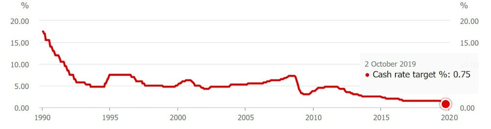
There are a number of variants of the “monetary policy doesn’t work” argument. The most basic is that the Reserve Bank has this year cut rates from 1.50% to 0.75% without any improvement to the Australian economy.
This is a textbook example of one of the classic logic fallacies known as “post hoc ergo propter hoc” (from the Latin, meaning “after this, therefore because of this”).
Put simply, it assumes the rate cuts have had no effect and doesn’t account for the possibility things might have been worse had there been no cuts.
Things might have been even worse. We’ll never know.
It also ignores what might have happened if the RBA had cut sooner. Again, we can’t know for sure. It is possible, though, to make an educated guess.
When to cut rates
Had Reserve Bank governor Philip Lowe acted, say, 18 months earlier to cut rates, he would have signalled that Gross Domestic Product growth was indeed lower than desired, that the sustainable rate of unemployment was more like 4.5% than 5%, and, most importantly, that he understood the need to act decisively.
That would have sent a powerful signal.
It would also have ameliorated the huge decline in housing credit that pushed down housing prices in Sydney and Melbourne by double digits.
That, in turn, would have prevented some of the weakening in the balance sheets of the big four banks that has occurred (witness this annual general meeting season).
All of this would have pumped more liquidity into the economy and put households in a much stronger position, likely leading to stronger consumer spending than we have seen.
Bank pass through
One gripe both the Reserve Bank governor Philip Lowe and federal treasurer Josh Frydenberg have had with the banks is their failure to fully pass through the RBA cuts.
It is true there is a problem with banks not being able to cut deposit rates below zero, and as a result having less scope to cut mortgage rates, which are majority funded from deposits.
But there are, of course, other ways monetary policy can work. The leading example is quantitative easing (QE).
This is where the central bank pushes down long-term interest rates by buying government and corporate bonds. At the same time this expands the money supply, thereby adding some upward inflationary pressure.
There is little reason to think such measures wouldn’t work.
The power of free money
Perhaps paradoxically, the closer interest rates get to zero the more powerful those rates may end up being.
To put it bluntly, if someone shoves a pile of money into your hand and asks almost nothing in return, you’re likely to use it. In fact, you would be pretty silly not to.
Suppose your mortgage rate really goes to zero – as has happened in Europe.
You might decide to redraw that and spend the money on a home renovation or some other productive purpose. Or you might decide to buy a more expensive house.
Such spending provides an economic boost.
The effect is all the more pronounced if people expect interest rates to be low for a long period of time. Aggressive cutting coupled with quantitative easing – which lowers long-term rates – signal just that.
But not only monetary policy
Just because monetary policy still has some effect at near-zero rates doesn’t mean we should pin all of our economic hopes to it.
A near consensus of economists have argued repeatedly for the use of more aggressive fiscal policy – including more infrastructure spending and more tax cuts.
Indeed, Philip Lowe has raised eyebrows by speaking so forthrightly on this issue. That doesn’t make him wrong, though.
There is little doubt the Reserve Bank should have acted much earlier to cut official interest rates. There is also a very good chance it will need to begin to use other measures such as quantitative easing in the relatively near future.
All of that says the Australian economy, like most advanced economies around the world, is in bad shape.
But it doesn’t mean monetary policy has completely run out of puff.
Author: Richard Holden, Professor of Economics, UNSW
Hold Your Horses! RBA Does Too…
The RBA held rates today, as expected, but their explanation is turning pretty sour as reality bites. Expect more downgrades and rate cuts ahead, just a matter of time.
I also find it amazing that unlike UK, USA, and NZ there is no streamed press conference nor questions from the media after the announcement. The RBA continues to be more covert than its peers and less exposed to questions about its policy.

At its meeting today, the Board decided to leave the cash rate unchanged at 0.75 per cent.
While the outlook for the global economy remains reasonable, the risks are tilted to the downside. The US–China trade and technology disputes continue to affect international trade flows and investment as businesses scale back spending plans because of the uncertainty. At the same time, in most advanced economies, unemployment rates are low and wages growth has picked up, although inflation remains low. In China, the authorities have taken steps to support the economy while continuing to address risks in the financial system.
Interest rates are very low around the world and a number of central banks have eased monetary policy in response to the persistent downside risks and subdued inflation. Expectations of further monetary easing have generally been scaled back over the past month and financial market sentiment has improved a little. Even so, long-term government bond yields are around record lows in many countries, including Australia. Borrowing rates for both businesses and households are also at historically low levels. The Australian dollar is at the lower end of its range over recent times.
The outlook for the Australian economy is little changed from three months ago. After a soft patch in the second half of last year, a gentle turning point appears to have been reached. The central scenario is for the Australian economy to grow by around 2¼ per cent this year and then for growth gradually to pick up to around 3 per cent in 2021. The low level of interest rates, recent tax cuts, ongoing spending on infrastructure, the upswing in housing prices in some markets and a brighter outlook for the resources sector should all support growth. The main domestic uncertainty continues to be the outlook for consumption, with the sustained period of only modest increases in household disposable income continuing to weigh on consumer spending. Other sources of uncertainty include the effects of the drought and the evolution of the housing construction cycle.
Employment has continued to grow strongly and has been matched by strong growth in labour supply, with labour force participation at a record high. The unemployment rate has remained steady at around 5¼ per cent over recent months. It is expected to remain around this level for some time, before gradually declining to a little below 5 per cent in 2021. Wages growth remains subdued and is expected to remain at around its current rate for some time yet. A further gradual lift in wages growth would be a welcome development and is needed for inflation to be sustainably within the 2–3 per cent target range. Taken together, recent outcomes suggest that the Australian economy can sustain lower rates of unemployment and underemployment.
The recent inflation data were broadly as expected, with headline inflation at 1.7 per cent over the year to the September quarter. The central scenario remains for inflation to pick up, but to do so only gradually. In both headline and underlying terms, inflation is expected to be close to 2 per cent in 2020 and 2021.
There are further signs of a turnaround in established housing markets, especially in Sydney and Melbourne. In contrast, new dwelling activity is still declining and growth in housing credit remains low. Demand for credit by investors is subdued and credit conditions, especially for small and medium-sized businesses, remain tight. Mortgage rates are at record lows and there is strong competition for borrowers of high credit quality.
The easing of monetary policy since June is supporting employment and income growth in Australia and a return of inflation to the medium-term target range. Given global developments and the evidence of the spare capacity in the Australian economy, it is reasonable to expect that an extended period of low interest rates will be required in Australia to reach full employment and achieve the inflation target. The Board will continue to monitor developments, including in the labour market, and is prepared to ease monetary policy further if needed to support sustainable growth in the economy, full employment and the achievement of the inflation target over time.
The Credit Impulse Dies Some More [Video]
The latest RBA and APRA stats reveals credit momentum is still slowing, and the full year results from ANZ shows the stresses in the system. And weaker building approvals are not helping either.
Credit Impulse Dies Some More
We are getting to the rub now with the RBA releasing its Credit Aggregate data to end September 2019. This is loan stock data, reflecting the net effect of new loans coming on, old loans repaid, refinancing, and any reclassification which occurred in the month.
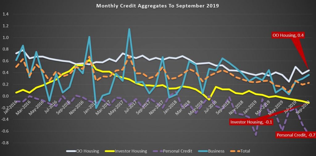
Over the month of September, total credit grew by 0.2%, with housing also at 0.2%, business at 0.4% and personal credit down another 0.7%. Owner occupied lending was a little firmer, but investment lending faded again.
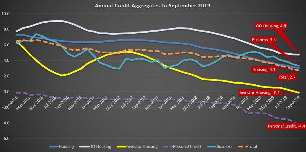
For the year ending, total credit grew by 2.7%, the lowest since June 2011, Housing at 3.1%, the lowest at least since 1977, and business at 3.3%. Personal credit fell 4.4% over the year.
Given the strong link between home prices and housing credit, this suggests home prices will continue weaker ahead. And this, after all the recent adjustments to lending standards and rates.
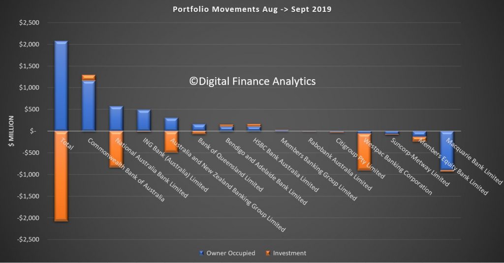
The APRA data also shows some swings between lenders during the month (or reclassification, we cannot tell). NAB, ANZ and Westpac all dropped their investment loan balances, while Macquarie dropped their owner occupied loans.
RBA Rose Tinted Specs On The Blink
The RBA minutes for October are decidedly bearish, clearly the battery in their rose-tinted specs as run down, revealing the mounting risks in the economy. Probably more risks ahead, more cuts and the proverbial QE in some form…

International Economic Conditions
Members commenced their discussion of global economic conditions by noting that heightened policy uncertainty was affecting international trade and business investment. This had continued to be apparent in a range of indicators, including new export orders and investment intentions. Conditions in the manufacturing sector had remained subdued, partly because of ongoing US–China trade tensions. These tensions had led to a contraction in bilateral trade between the United States and China, which was resulting in the diversion of some activity to other economies. Members noted that the trade and technology disputes continued to pose significant downside risks to the global economic outlook.
In general, conditions in the services sector had been relatively resilient in most advanced economies, supported by strong labour market conditions. Employment growth had continued to outpace growth in working-age populations, unemployment rates had remained at low levels and wages growth had risen. Nevertheless, inflation had remained low, although core inflation had picked up in the United States in recent months.
In the United States, GDP growth appeared to have slowed a little further in the September quarter. Growth in core capital goods orders and investment intentions had declined, whereas growth in consumption had remained robust. In the euro area, the weakness in output growth in the June quarter had been broadly based. Industrial production had fallen, particularly in Germany, and investment intentions had remained below average. In Japan, exports had declined further, although output growth in the September quarter had been supported by above-average household spending ahead of an increase in the consumption tax in October.
In east Asia, export volumes had been flat for several months. Other indicators of activity, such as industrial production and surveys of manufacturing conditions, had shown tentative signs of stabilising. Growth in output had also slowed in India, driven by weakness in consumption. Members noted that the political unrest in Hong Kong had affected economic activity there to a significant extent.
In China, a range of indicators suggested that the pace of economic activity had slowed since the start of the year. Economic indicators remained subdued in August, although they had recovered a little from broad-based weakness in July. Growth in industrial production and retail sales had edged higher in August, and fixed asset investment growth had been broadly unchanged. Conditions in housing markets also appeared to have softened. In response to the slowing in activity, the authorities had announced further measures to ease policy in September. Chinese demand for imported iron ore and coal had increased, supported by ongoing investment in infrastructure.
The iron ore benchmark price had continued to be volatile since the previous meeting. Members noted that supply concerns in the iron ore market had eased somewhat, and ongoing strength in Chinese steel demand had been met by an increase in iron ore imports. Oil prices had also been volatile, with the attacks on oil infrastructure in Saudi Arabia having disrupted oil supply and exacerbated uncertainty in the region.
Domestic Economic Conditions
Members noted that the main domestic economic news over the previous month had been the release of the national accounts data for the June quarter and updates on the labour and housing markets. On balance, the data had pointed to a continuation of recent trends.
The national accounts reported that the Australian economy had grown by 0.5 per cent in the June quarter. Year-ended growth had slowed to 1.4 per cent, the lowest outcome in a decade. Nevertheless, there had been a pick-up in quarterly GDP growth over the first half of 2019 compared with the second half of 2018. The pick-up had been driven by stronger growth in exports, led by exports of resources and manufacturing goods. Members noted that export demand was being supported by the lower level of the Australian dollar. Public demand had also been growing strongly, partly because of spending on the National Disability Insurance Scheme. Members observed that the drought had continued to affect the rural sector to a significant extent and that, as a result, farm output was expected to remain weak over the following year.
Growth in household disposable income had been subdued. Strong growth in income tax paid by households had been a contributing factor, as had been low growth in non-labour income, partly reflecting the effects of the drought on the farm sector. By contrast, strong employment growth had boosted growth in labour income.
Consistent with the ongoing low growth in household disposable income, household consumption had increased by only 1.4 per cent over the year to the end of June. Members noted that there had not yet been evidence of a pick-up in household spending following the recent reductions in the cash rate and receipt of the tax offset payments, although they acknowledged that it may be too early to expect any signs of a pick-up. Retail sales had remained subdued in July and car sales had decreased in August. Despite weak reported retail sales conditions generally, on a slightly more positive note some contacts in the Bank’s liaison program had reported a mild pick-up in retail sales since July. Responses to consumer surveys in September had suggested that, on average, households planned to spend around half of their lump-sum tax payments, broadly in line with what had been assumed in the Bank’s most recent forecasts.
The residential construction sector had contracted further and this was expected to continue for some time. The decline in dwelling investment in the June quarter was greater than had been expected a few months earlier. Higher-density approvals had declined in July, to be at their lowest level in seven years; detached approvals had also declined in July. The Bank’s liaison program had continued to report weak pre-sales for higher-density developments. Taken together, this information implied that dwelling investment would decline further over coming quarters.
The turnaround in the established housing market had continued in September. Housing prices had increased further in Sydney and Melbourne, and auction clearance rates had remained high in both cities. The pace of growth in housing prices had also picked up in some other capital cities in recent months. However, housing turnover had remained low.
Business investment had decreased a little in the June quarter, driven by a decline in non-residential construction outside the mining sector. Nevertheless, the outlook for non-mining business investment remained favourable, supported by investment in infrastructure. Mining investment had picked up largely as expected. Members noted that mining investment was expected to continue to increase gradually, supported by projects both to sustain and to expand production. Survey measures of business conditions had remained around average in August; members noted that conditions in retailing were reported to have been very weak, while conditions in the mining industry had remained well above average.
Conditions in the labour market had continued to be mixed. Employment growth in August had remained stronger than growth in the working-age population, and the employment-to-population ratio had reached its highest level since late 2008. Employment had increased by 2½ per cent over the preceding year, the third successive year of strong employment growth. The participation rate had also increased to another record high. Members noted that the strong demand for labour had been met by an equally strong increase in supply. The unemployment rate had been around 5¼ per cent since April and the underemployment rate had remained above its recent low point. Looking ahead, job vacancies and advertisements had declined, suggesting that employment growth would probably moderate over the subsequent few quarters. Members noted that the ongoing subdued growth in wages implied that there continued to be spare capacity in the labour market.
Financial Markets
Members noted that financial conditions remained accommodative internationally and in Australia. Several major central banks had eased policy in September and market pricing implied that market participants expected the global economic expansion to be sustained by an extended period of policy stimulus. Expectations of further monetary easing had been partially scaled back in response to tentative signs of progress in the trade and technology negotiations between the United States and China and some better-than-expected US economic data. These developments had also supported the prices of equities and corporate bonds.
As expected, the US Federal Reserve had reduced its policy rate again by 25 basis points in September. The Federal Reserve had noted that, although the US economy had remained strong, easier policy was warranted given muted domestic inflation pressures, a weakening in global activity and persistent downside risks. Members of the Federal Open Market Committee did not anticipate a prolonged easing cycle, but continued to signal that they were willing to ease policy further if needed to sustain growth and meet the Federal Reserve’s inflation objective. Market pricing suggested that the federal funds rate was expected to decline by a further 50 basis points or so by mid 2020, which was a little less than had previously been anticipated.
The European Central Bank (ECB) had delivered a package of stimulus measures in response to inflation being persistently below the ECB’s target, protracted weakness in economic growth and continued downside risks. The package included cutting the ECB’s policy rate by 10 basis points to –0.5 per cent, exempting a portion of banks’ excess reserves from negative deposit rates, committing to not lifting rates until inflation returned sustainably to target, renewing purchases of government and private sector securities, and easing the conditions of the targeted long-term refinancing operations designed to encourage banks to lend to the private sector.
The People’s Bank of China had provided additional but targeted monetary stimulus, further cutting its reserve requirements, with larger adjustments for some smaller banks that are important providers of finance to small businesses. Chinese banks had also lowered the benchmark lending rate for corporate borrowers slightly.
Government bond yields in major markets had risen a little, with yields in Australia following suit. Nonetheless, bond yields remained very low, with a large portion of bonds in Europe and Japan trading at negative yields. Members noted that a sizeable proportion of the investors holding these negative-yielding bonds were constrained by their mandates or regulatory requirements, including asset managers, banks, insurance companies and pension funds.
Members noted that financing conditions for corporations remained favourable globally. Equity prices had remained close to recent peaks, spreads on corporate bonds were low and issuance volumes had been strong. In Australia, the cost of capital for corporations had been quite stable for some years, although more recently it had declined a little. Members also discussed hurdle rates for business investment, which had not changed much over recent times.
Major exchange rates had generally been little changed over September, with the US dollar having appreciated over the preceding two years or so on a trade-weighted basis. The Chinese renminbi had stabilised after its earlier depreciation, while the Japanese yen had depreciated, consistent with some easing of concerns about global risks. The Australian dollar had been little changed and remained around its lowest level in recent years.
In Australia, borrowing rates for households and businesses, as well as banks’ funding costs, were at historically low levels. Housing loan approvals to both owner-occupiers and investors had increased in the three months to August, consistent with stronger conditions in some established housing markets. However, members noted that this increase in approvals had not yet translated into faster growth in housing credit. The pace of growth in housing credit for owner-occupiers had been fairly steady since the beginning of the year and the stock of housing credit for investors had continued to decline a little.
Financial market pricing indicated that a 25 basis points reduction in the cash rate was largely priced in for the October meeting, with a further reduction expected by mid 2020.
Financial Stability
Members were briefed on the Bank’s regular half-yearly assessment of the financial system.
Globally, investors were accepting low rates of compensation for bearing risk, despite the increased chance of significantly weaker economic growth. Members noted that a sharp slowdown in global growth could result from an escalation of the US–China trade and technology disputes or geopolitical tensions in the Middle East, Hong Kong or the Korean peninsula. Central banks had eased monetary policy in response to the potential for weaker growth, and additional easing was expected by markets, leading to falls in long-term government bond yields. Despite the increased uncertainty, risk premiums were low and in some cases had fallen further. The lower risk-free interest rates and low term, credit and liquidity risk premiums had seen many asset prices increase further. Any shock that caused markets to increase risk premiums or revise upwards expectations of future policy rates, such as a pick-up in inflation without accompanying stronger growth, could see a broad range of asset prices fall. Given debt levels were high in some non-financial sectors in some economies, a fall in asset prices could result in financial stress for some businesses and households, which could spill over to financial institutions.
Members observed that there had been strong growth in corporate debt in the United States, France and Canada, particularly lower-quality debt. Members noted that borrowers whose credit ratings fell below investment grade, and who relied on market-based finance, could face difficulty accessing funding, given many investors’ mandates were constrained by credit ratings. The interaction of high sovereign debt and less resilient banks in Japan and some European economies was also seen as a risk. However, in the United States and the United Kingdom, the resilience of the banking system had increased as profitability had improved.
Corporate debt in China had increased sharply over the previous decade, although in relation to GDP it had declined recently in response to policy measures to promote deleveraging. These measures included closing some unprofitable state-owned firms, restructuring some debt, reducing the size of non-bank financing and reducing non-banks’ interactions with banks.
In Australia, near-term risks related to the housing market had eased in the preceding few months with a turnaround in housing prices in Sydney and Melbourne. Prices in those cities had fallen by a little under 10 per cent over the preceding 18 months, reducing the housing equity of households and resulting in a small share with negative equity. The recent increase in housing prices in those cities had reduced the risk of large increases in negative equity, which could result in losses for lenders if declines in income reduced households’ ability to meet debt repayments. Half of all loans in negative equity were in Western Australia and the Northern Territory, where housing price declines had persisted over the previous few years. Members noted that the rate of mortgage arrears in Western Australia had increased by more for riskier types of lending, including lending with smaller deposits, higher repayments relative to income, and loans to investors and self-employed borrowers.
Despite the high level of household debt in Australia relative to other countries, the risks from household debt appeared to be mostly contained. While the share of mortgages in arrears had continued to rise, it remained at a low rate relative to many other countries and in absolute terms. In addition, the quality of new lending had increased in recent years. The shares of loans with high loan-to-valuation ratios and with interest-only repayment terms had declined following a focus by regulators on this higher-risk lending. Further, members noted that households continued to have large prepayments on their housing debt. In aggregate, mortgage prepayments were equal to two-and-a-half years of repayments. However, while one-third of borrowers had prepayments exceeding two years of mortgage repayments, a slightly lower share had very little or no buffers. Of these, a little less than half appeared more likely to be vulnerable to shocks to their ability to meet their mortgage payments.
The resilience of Australian banks had increased since the financial crisis. Banks had largely completed their transition to their higher ‘unquestionably strong’ capital ratios. Banks’ resilience would increase further with the introduction by the Australian Prudential Regulation Authority of a Loss Absorbing Capacity (LAC) regime, which will require banks to raise an additional 3 percentage points of capital by 2024. Members observed that banks were already issuing new Tier 2 securities to meet their LAC requirements. Banks’ profitability had declined a little over the prior year or two, although banks remained highly profitable. The increase in housing arrears had resulted in a small decline in banks’ overall asset quality, although asset quality remained high. Rates of non-performing business loans were a little below rates for housing loans.
Members also discussed non-financial risks facing the financial system. Members noted that cyber risks, and IT risks more broadly, were increasing as technology systems become more complex and embedded in all operations. Members also noted that climate change presented a risk to financial institutions. While extreme weather events were thought unlikely to produce large losses for the financial system as a whole, at least at present, losses could be larger in future if financial institutions do not manage the risks carefully.
Considerations for Monetary Policy
In considering the policy decision, members observed that the risks to the global growth outlook remained tilted to the downside. The trade and technology disputes between the United States and China were affecting international trade and investment, as businesses scaled back their spending plans in response to increased uncertainty. In China, the authorities had taken further steps to support the economy, while continuing to address risks in the financial system. In most advanced economies, inflation remained subdued despite low unemployment rates and rising wages growth.
In this context, global interest rates had continued to decline, with the central banks in the United States and Europe reducing interest rates in the previous month. Further monetary easing was widely expected, as central banks continued to respond to the downside risks to the global economy and subdued inflation. Long-term government bond yields were close to record lows in many countries, including in Australia. Borrowing rates for both businesses and households were at historically low levels, and the Australian dollar was at its lowest level in recent years.
Members considered the case for a further easing in monetary policy at the present meeting, to support employment and income growth and to provide greater confidence that inflation would be consistent with the medium-term target. Members noted that the Bank’s most recent forecasts suggested that the unemployment and inflation outcomes over the following couple of years were likely to be short of the Bank’s goals. The most recent run of data had not materially altered this assessment and, on balance, had been on the softer side. The ongoing subdued rate of wages growth also suggested that the economy still had spare capacity. There was therefore a case to respond to the general outlook with a further easing of monetary policy.
Members were mindful, however, that monetary policy was already expansionary and that the lower exchange rate was also supporting growth. They acknowledged that these factors and the recent tax cuts could combine to boost growth by more than their individual effects would imply, especially given the context of the mining and established housing sectors seeming to have reached turning points. At the same time, members recognised that it was possible that the effects may be smaller than expected and the global risks were to the downside.
Members also considered the argument that some monetary stimulus should be kept in reserve to address any future negative shocks. However, that argument requires changes in interest rates to be the key driver of demand, rather than the level of interest rates, which experience has shown to be the more important determinant. Members concluded that the Board could reduce the likelihood of a negative shock leading to outcomes that materially undershot the Bank’s goals by strengthening the starting point for the economy.
The Board’s discussions also focused on the ongoing strength in employment growth. The period of strong employment growth had not reduced spare capacity in the labour market significantly. Almost all of the strength in employment growth over the preceding three years had been matched by higher participation, so there had been little progress on reducing unemployment and underemployment. It was also possible that participation was rising partly in response to weak growth in incomes. Moreover, employment growth was forecast to slow over the period ahead.
Members also discussed the possibility that policy stimulus might be less effective than past experience suggests. They recognised that some transmission channels, such as a pick-up in borrowing or the effect on the home-building sector, may not be operating in the same way as in the past, and that the negative effect of low interest rates on the income and confidence of savers might be more significant. Notwithstanding this, transmission through the exchange rate channel was still considered likely to work effectively, and evidence suggested that the positive effects of lower interest rates on aggregate household cash flows via lower debt repayments was likely to support household spending, given that household interest payments exceed receipts by more than two to one.
Members also noted that the housing market and other asset prices might be overly inflated by lower interest rates. Members acknowledged that asset prices were part of the transmission mechanism of policy, including by encouraging home building. By themselves, higher asset prices were considered unlikely to present a risk to macroeconomic and financial stability. This assessment would need to be reviewed if rapidly increasing asset prices were accompanied by materially faster credit growth, weak lending standards and rising leverage. Although household debt was still considered high, members saw only a limited risk of excessive borrowing at the current juncture: household disposable income growth (and thus borrowing capacity) is weak; the memory of recent housing price falls is still fresh; and banks are still quite cautious in their appetite to lend. Nonetheless, members assessed that close monitoring of this risk was warranted.
Members concluded that these various factors did not outweigh the case for a further easing of monetary policy at the present meeting. Taking into account all the available information, including the reductions in interest rates since the middle of the year, the Board decided to lower the cash rate by a further 25 basis points. Members judged that lower interest rates would help reduce spare capacity in the economy by supporting employment and income growth and providing greater confidence that inflation would be consistent with the medium-term target. Members also noted the trend to lower interest rates globally and the effect this was having on the Australian economy and inflation outcomes.
Members judged it reasonable to expect that an extended period of low interest rates would be required in Australia to reach full employment and achieve the inflation target. The Board would continue to monitor developments, including in the labour market, and was prepared to ease monetary policy further if needed to support sustainable growth in the economy, full employment and the achievement of the inflation target over time.
The Decision
The Board decided to lower the cash rate by 25 basis points to 0.75 per cent.
RBA On ‘Emergency Liquidity Injections’
The RBA released “Research Discussion Paper – RDP 2019-10 Emergency Liquidity Injections” by Nicholas Garvin.

Here is the non-technical summary.
Understanding liquidity crises has long been, and will probably long be, an important objective for economic policymakers. Liquidity risk is inherent to banking systems because banks fund long-term assets (like mortgages) with short-term and at-call debt (like deposits). This process benefits the economy by making more credit available for households and businesses. However, it also generates the risk that if short-term debtholders withdraw their funds en masse, banks are unlikely to be able to pay them. This paper contributes to the research literature that studies how a policymaker can handle such a situation, which broad monetary stimulus is not designed for, by modelling the scenario faced by the United States and other global financial centres in late 2008. This type of situation appears highly unlikely in Australia in the foreseeable future.
The model depicts a banking system that is solvent, but a system-wide withdrawal by debtholders leaves banks with short-term payment obligations that exceed their available funds (i.e. their liquidity). It is then in the policymaker’s interests to inject liquidity into the banking system, which can prevent bank failures and the harm to the economy that would likely follow. However, injecting liquidity incentivises banks to take more liquidity risk the next time around, which makes future liquidity crises more likely. This paper compares different types of liquidity injection policies by where they sit in the trade-off between the perverse incentives generated, and the ability to support the banking system during a crisis.
To address the subject, I develop a game-theoretic model in which banks decide how many liquid assets to hold as protection against funding withdrawals. Banks consider the losses they would suffer if a crisis eventuated, which depend on the type of liquidity injection policy implemented by the policymaker. If a crisis eventuates, the type of policy also influences how the crisis unfolds. By placing a particular type of policy into the model, we can therefore analyse that policy’s influence on banks’ risk-taking decisions and on crisis outcomes. The model replicates some features of liquidity injection policies highlighted previously in the research literature. It also generates two new insights, which are the paper’s main contributions.
The first insight is that, if the policymaker injects liquidity by lending to banks, there is an indirect benefit of requiring them to provide collateral. The benefit arises through the (secondary) markets for the securities that the policymaker accepts as collateral. In the model, the crisis is characterised by falling prices in these markets, driven by selling pressure from the banks that need more cash. However, banks cannot sell securities that they are providing as collateral. Collateral requirements can therefore alleviate ‘fire sales’ in these markets, which benefits other banks through the higher market prices. In aggregate, the banking system ends up better off after the crisis, but, for each individual bank, there is no increase in the return to taking more liquidity risk.
The second insight is about whether a policymaker can disincentivise risk-taking by charging high ‘penalty’ interest rates on its emergency lending. Farhi and Tirole (2012) argue that, regardless of the effects on banks’ incentives, once a crisis occurs, the policymaker will then offer low rates. This is because the risk-taking that caused the crisis has already taken place, and charging banks penalty rates could now put them in further distress. Therefore, banks view any claims by the policymaker that it would charge penalty rates in a crisis as not credible, so such claims are powerless to influence risk-taking. I present a counterargument: penalty rates can be credible if the emergency loans are long term. In the crisis I model, banks are in liquidity distress but they are still solvent (i.e. they have not run out of capital). This means they will have no trouble making the repayments once liquidity conditions in the banking system improve. Charging banks penalty rates on long-term loans during a crisis will therefore not put them in further distress, which gives penalty rates more credibility.